Monday, March 20, 2017

Kaggle Project: Two Sigma Connect Rental Properties

Working on a Kaggle project now (https://www.kaggle.com/c/two-sigma-connect-rental-listing-inquiries) about predicting interest levels for housing in NYC. The data includes images, presumably to encourage application of computer vision, and text descriptions...so much stuff. These kinds of projects would require huge amounts resources and time to actually do well, but I will document my stab at it here. I don't intend to get too obsessed with this project, as I would if I saw it as a litmus test of my analytical abilities, and all I'm hoping is to learn a couple things while working on it. 

Geographical Analysis of High, Med, Low Interest Listings


Getting started, I did some general exploratory data analysis. Here are the listings separated by interest level (of which there are only three: high, medium, low) overlaid onto a map of NYC. I took out a couple geographical outliers, but otherwise unaltered.  


Already, I can see how complicated this project could get. There are no indications of high interest listings clustering around a particular area, and the cartesian coordinates of the listings on the map probably are not going to help much in the classification. The high interest listings may seem sparser only because they have the fewest data points. For this location data to be useful in classifying, some inventive (and very detailed) feature engineering will be required. And that will require a lot of....manual work and analysis....


Interest Level to Price Relationship

Price was also included in the dataset. Intuitively, I expect that price data should matter a lot when it comes to interest level. From my personal experience looking for apartments, a large portion of the people who rent in the city are young professionals who don't have a family. Another guess is that these people all make around the same amount of money, and interest level should be intense for the nicer apartments in the 2k~3k range. Obviously, there are going to be listings much higher and lower than that, which do not attract the same amount of interest. The cheaper listings being in dangerous neighborhoods, and the expensive ones being out of reach for the majority of customers. That means the relationship of interest to price should be non-linear. The relationship could be linear after accounting for several factors, like location, etc. 


Sunday, December 6, 2015

Kaggle Competitions

So there have been a lot of changes in my life since my last blog post. Since graduating from graduate school in May, I have begun working at a consulting firm in Chicago, where my work is related mostly to quantitative finance and auditing financial models so to speak. I am finding that industry is a lot different from academia, and I now have a lot more time to myself than I used to have in graduate school. 

So I've begun working on Kaggle projects in my free time. The one I am currently working on is the Walmart one. 

I have a couple of ideas that I want to test out, which are:
  1. Nested Logit Regression
  2. Multinomial Logit Regression


Wednesday, July 1, 2015

Pairs Trading: Avellaneda & Lee (2008)

This blog post is about the famous Avellaneda & Lee (2008) paper on statistical arbitrage, which presented a method to build a profitable 'pairs trading' strategy. I decided to try the method suggested in the paper myself, and see if I can come up with something profitable. According to the paper, we can model two stocks with correlated movements using the following model:

\begin{align}
\underbrace{ \log \left(\frac{P_t}{P_0} \right)}_{\text{relative value of P}} = \alpha (t - t_0) + \beta \underbrace{ \log \left(\frac{Q_t}{Q_0} \right)}_{\text{relative value of Q}} + \underbrace{X_t}_{\text{cointegration residual}} && \text{...for $t = \{1,2, \cdots n \}$} \label{eq:cointegration}
\end{align}

If $X_t$ is a mean-reverting and stationary process, then we say that the two stocks $P$ and $Q$ are cointegral. We see that the regression is not the same as regressing the 1-day returns of stock P onto stock Q:

\begin{align}
\log \left( \frac{P_t}{P_{t-1}} \right) = \hat{\alpha} + \hat{\beta} \log \left( \frac{Q_t}{Q_{t-1}} \right) + \epsilon_t && \text{...for $t = \{1,2, \cdots n \}$}
\end{align}

However, we can link these two equations together, since:

\begin{align}
\log \left( \frac{P_n}{P_0} \right) &= \sum_{i=1}^{n} \log \left( \frac{P_i}{P_{i-1}} \right) \\
&= \sum_{i=1}^n \hat{\alpha} + \hat{\beta} \sum_{i=1}^n \log \left( \frac{Q_i}{Q_{i-1}} \right) + \sum_{i=1}^n \epsilon_i \\
&= \hat{\alpha} \cdot n + \hat{\beta} \log \left( \frac{Q_n}{Q_{0}} \right) + \sum_{i=1}^n \epsilon_i
\end{align}

So we get the following equality:

\begin{align}
X_t = (\hat{\alpha} - \alpha) n + (\hat{\beta}-\beta) \log \left( \frac{Q_n}{Q_{0}} \right) + \sum_{i=1}^n \epsilon_i
\end{align}

Which is not a very significant result, but it was fun anyway. It's noteworthy that we obtain different OLS estimates for $\alpha$ and $\beta$ under the two regressions, and this can be calculated explicitly with the OLS equations.

Case Study: AAPL and GOOG

So let's choose two stocks we all know to be highly correlated; Apple and Google. Below are the price series for the two stocks:


Now, we implement the equation above substituting AAPL for $P$ and GOOG for $Q$. Below is the regression output:


It's apparent that this regression is highly significant with the low P-values, but the R-squared value is quite low. We inspect the plot of the cointegration residuals, and look for stationarity: 

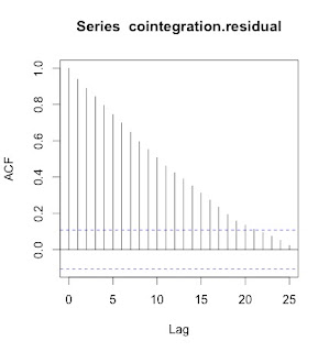
The residuals show signs of normality, as the QQ plot shows. We look at the ACF plot and perform an Augmented Dickey-Fuller test for unit roots on this process. 


Our ADF test indicates that the we cannot reject the null hypothesis of non-stationarity at the 18.4% level. Which means that at the 5% level, our process is not stationary and therefore AAPL and GOOG are not cointegral. So even though these two stocks are highly correlated, they are not cointegral.


AR(1) Filtering of the Cointegration Residuals

It's very peculiar that our ACF plot shows such high levels of persistence in the cointegration residuals. It looks like a plot of a AR1 model. It would be interesting to know if we can obtain stationarity in the residuals if we subtract this AR1 component. 

So first we set up the AR1 model:

\begin{align} \text{cointegration residual}_{t+1} \sim \beta * \text{cointegration residual}_t + \epsilon_t \end{align}

The intercept is deliberately not included in the model. Below is the regression output:


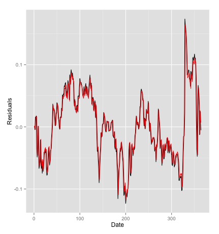
Wow. An R-squared of .8927? That is indicative of a very high degree of linearity. Here's a plot of the actual values versus forecasted; the red line is the prediction: 

Note that to construct the red line I'm just multiplying the previous day's actual value with the coefficient obtained from the AR1 regression, 0.945. 

After getting this, we now obtain the filtered residuals:
And this process turns out to be stationary at the 1% level:


Conclusion

Although AAPL and GOOG are not cointegral in the traditional sense, we can still obtain stationarity in the residuals after filtering for a AR1 process (which we assume to be deterministic). It's interesting to consider if this implies that we can still implement a profitable pairs trade on these two stocks.  

Avellaneda and Lee (2008) suggest a trading strategy where we go long on $\text{\$1}$ of AAPL and short on $\beta$ dollars of GOOGL when our stationary residual is low, and vice versa when our residual is high. This means if we are able to predict the cointegration residual, we can make a profitable portfolio. 

In the next post I will turn my attention now to modeling and forecasting the cointegration residuals, and backtesting some strategies for AAPL and GOOG. 

Aside: Vasicek Model 

A popular way to model mean-reverting processes is the Vasicek Model:

\begin{align}
dx_t = k(m - x_t)dt + \sigma dW_t
\end{align}

Where $k$ signifies the speed of mean reversion. $m$ signifies the long-run mean, $\sigma$ signifies the instantaneous volatility, and $dW$ is a Brownian motion process. The Vasicek Model belongs to a class of stochastic processes called Ornstein-Uhlenbeck Processes, meaning that they revert to some long-run mean after a while.

We calibrate our above time series to the Vasicek Model. Calibration can be done via Least-Squares. Let's discretize our stochastic differential equation first:

\begin{align}
dx_t &= k(m - x_t)dt + \sigma dW_t \\
x_{t+1} - x_t &= k(m - x_t)dt + \sigma \sqrt{dt} \epsilon_t \\
\epsilon_t &\sim N(0,1)
\end{align}

Now rearrange algebraically,
\begin{align}
\underbrace{x_{t+1}}_{y} &=  \underbrace{k*m*dt}_{\alpha} + \underbrace{x_t(1 - k*dt)}_{\beta x} + \underbrace{\sigma \sqrt{dt} z_t}_{\epsilon}
\end{align}

With the last equation we see the linear regression equation. Thus we regress $y_{t+1}$ on $y_{t}$ and retrieve our parameters through the following transformation on our coefficient estimates:

\begin{align}
\alpha &= k*m*dt \\
\beta &= 1 - k * dt \\
\sigma & = \frac{S.D. \epsilon}{\sqrt{dt}}
\end{align}

Vasicek Model Monte-Carlo Simulation

After calibrating the spread to the Vasicek Model with the above procedures, we obtain the following parameters: $k = 9.56$, $m = -0.0037$, $\sigma = 0.206$. We can simulate some realizations of this Vasicek Process to make sure these parameters sound reasonable. The red line is the Monte-Carlo simulation, and the black line is the actual cointegration residual:

The model appears to capture properties of the cointegration residuals fairly well.

References

Avellaneda & Lee. (2008). Statistical Arbitrage in the U.S. Equities Market.


Thursday, July 3, 2014

Types of Options

Different Types of Options

Last time we looked at the basic idea of what an option is. There are many different types of options, and new ones can be imagined easily with some creativity.

In the academic world, there are two main types of options that have have been studied extensively. These options are called "plain vanilla" options, and they are also traded frequently on the options exchanges in the United States:

  1. European Option - an option contract that can only be exercised at maturity.
  2. American Option - an option contract that can be exercised at any time up to maturity. 

 In addition to the above types of options, there are a couple more that have received attention in academia. The options below are called "exotic" options, and they are not traded frequently on exchanges. Most of the time, exotics are traded "over-the-counter" in bilateral contracts:

     3.  Asian Option - the payoff at maturity depends on the average price of the underlying asset.
     4.  Barrier Option - if the price of the underlying asset hits some pre-specified "barrier" price, then the option contract is voided.

Note that exotics can also be European or American options. For example, you can make an Asian European option, or an American Barrier option, and vice versa. 

Techniques for Pricing the Basic Options

The plain vanilla European and American options are the most basic, and also the most traded options. The techniques used to price European and American options can be extended in many cases to price exotic options. Thus it is important that we pick up the basic toolkits to price these options before we move forward. There are a number of methods, each having its own advantages/disadvantages, and intricacies that will take some time to fully master. The basic ones that I will cover in future posts are:
  1. Monte-Carlo Simulations - simulate price paths for the underlying asset (stock price) using random numbers. 
  2. Black-Scholes PDE - a set of three equations that can easily be calculated by hand with a scientific calculator gives us the price for a European option.
  3. Black-Scholes PDE via the Finite Element (or Difference) Method - a numerical way of calculating the BS PDE. Requires some computational power and number-crunching.
  4. Binomial Model - used very widely in industry, it is one of the most resilient ways of pricing options.  

Methods Used to Price Options


One thing to note is that some of the methods listed above cannot be used to price American options. The reason for this comes from complications that arise due to the American Option being exercisable at any time.

In the following posts, we will start looking at these basic methods used to price options one-by-one. It might be worthwhile to note that in some cases, there are very clear "winners" as to which one is the best method to use. The reason why we still study the other methods is because they "might" become handy in other situations. My personal take is to look at this whole "option pricing" ordeal as a mathematical problem - the solution to which is mathematically interesting, but not always practical.

Option Pricing is not Physics

I will just add a small disclaimer for those of us who have received some training in the classical physics that option pricing "models" are not "true" in the sense that they are not made to reflect reality. Due to the complexity involved with the models use to price options, its easy to quickly lose track of this fundamental truth. Unlike "real engineering," where we in many cases we start of with the universal Newton's Laws etc., some fundamental theorem that has been tested to be true in a controlled environment millions of times before, the fundamental assumptions made in "financial engineering" are shaky estimations at best. Thus, many students - myself included - will find the lack of precision in such financial models to be frustrating when they start studying them. What's the point in building models that nobody can prove are accurate? Indeed, it's a cavernous business from the very beginning and some will say that it's more of an art than it is a science.

Saturday, June 28, 2014

Financial Engineering 101: What is an Option?

It's been a while since my first post. Since my last blog post I have moved to Tokyo for my summer internship, and this has been a source for many novel experiences. On a bright note, my current internship has given me some new insights on what is happening at the forefront of the financial industry, which I would like to contemplate on and share here.


Today I will discuss the "Option." It is the most basic and fundamental type of product in a class of financial instruments called "Derivatives." Personally, I would consider Robert Merton's 1973 paper deriving the Black-Scholes Equation on pricing derivatives to be the birth of financial engineering. As such, it is the central piece of any education in financial engineering.
While initially the method on how to "price" an option may seem of trivial importance, there is an enormous and extensive literature on how to accomplish this, many of which is covered in a financial engineering education. I will go into some depth on this in my later posts, but first lets go over the key concepts.

Basic Set-Up

An option (in finance) is, just like the name implies, an "option" to either buy or sell a stock at some pre-specified future date. This means that it's a contract that gives whoever is buying the option the right  - but not an obligation - to buy/sell the stock in the future. The two basic types are the call and put, with the call option being the right to buy and the put being the right to sell.

"Call Option" Contract


Example Problem

Forget the Black-Scholes and any other formulas for now - lets think logically how we should "price" this thing. Given that:
  • Lets say we are buying a call option on a share of Apple one year from now. 
  • Assume that Apple's share price right now is $92.
  • The "strike" of the option is also $\$92 $. This means that the option gives us the right to buy Apple stock one year from now for $92. 
  • Assume that somehow we know for certain that Apple's stock price one year from now will be $100. 
  • Let's say that 1-year treasury rates are 10%.
  • What is the most logical price for the Apple call option?

Solution: The No-Arbitrage-Pricing Concept

If we buy the Apple stock today and sell it at $\$100$ one year from now, we know for certain that we will make $\$8$ after one year. Thus from the concept of no-arbitrage-pricing, we would be given that the most logical price for the Apple call option should be the present value of $\$8 $. This is because if we buy the option at $\$8$ and exercise our right to buy the AAPL at $\$92$ one year from now and then sell it immediately for $\$100 $, we would neither make nor lose any money.
\begin{align} \text{Price of this Call} = \frac{8}{1+0.1} \end{align}

Note how the price of the option is dependent on a couple of things. Once we knew the price of the stock for the relevant times - as well as the risk-free interest rate - we were able to find out what the price for the option should be. This is why we say that options are derivative instruments. A derivative (conceptually) doesn't contain any new market information. It's price is (conceptually) solely dependent on the underlying asset, which in this case is the Apple stock. (I say "conceptually" because in the real world, its not quite this simple).

Okay, I hope that the above example gives a good explanation on what an option is, and also an inkling on how we price such financial instruments through the no-arbitrage-pricing concept. Note the many difficulties that we would encounter though, if we didn't make the assumptions that we made. In particular, how do you know the price of the stock one year from now with 100% certainty? What if the treasury rates changed? What if Apple went bankrupt before one year? Yes...indeed these are very important questions that have been asked before.

Why Study Options?

But even before we go into the details of how we price options in real life, lets ask ourselves why we need options at all and why we are even interested in learning how to price them. So far, I can come up with a couple reasons why we want to study options:

  1. Options are actually traded in large volumes on exchanges like the Chicago Board Options Exchange (CBOE) and the Chicago Mercantile Exchange (CME). Many traders make a living trading options on these exchanges, pocketing price discrepancies in the market. Therefore, from knowing this theory, you might actually be able to make some profit. Before you start trading options, you need to know the "correct price" so that you can determine whether the price on the market is too expensive or too cheap. 
  2. Options can be attractive instruments to keep in portfolios to hedge against certain risks. Some companies and asset management funds will invest in options to protect their portfolios. 
  3. The methods employed in pricing options can be transferred over to "price" different types of things. Real options are a tangential concept that stem from ordinary stock options. Such methods of modeling and valuing real options in the same way as stock options is beginning to change the way many companies are planning their businesses. Currently, only a select few companies at the forefront of new technologies have started employing these techniques in their businesses. Basically, it is the "cutting edge" technique for the valuation of companies in M&As, strategic decision making in consulting firms, etc. So if you want a job at a reputable consulting firm or an investment bank, I believe it to be possible that some knowledge on options will improve your chances on landing a gig!

Wednesday, May 28, 2014

The Expectation Maximization (EM) Algorithm


So what's a Gaussian Mixture?


Sometimes when we are analyzing data, we encounter situations when the probability density function of our data looks something like below:

Image and video hosting by TinyPic

As you might guess intuitively, this PDF looks like it is formed by two Gaussian distributions stuck together. Indeed, it was created from two Gaussian random variables of separate means and variances. You can kind of guess that the first distribution probably has a mean of around 5, while the second one has a mean of around 10. It also seems apparent that the variance of the first distribution is probably smaller than that of the second. 

Indeed, when I was generating the random variables that formed this PDF on Matlab, I used the parameters of $\mu_1=5$, $\sigma_1^2= 1$ for the first distribution, and $\mu_2=10$, $\sigma_2^2 = 2$ for the second distribution. 
But actually, there is one other parameter that I used to generate this weird PDF - it is the probability that we are in either of the states. That is, every time I draw my next random number, I choose to generate it with either of the two random number generators. But whether I choose the first or second generator is also random, and has some probability attached to it. I will call this parameter $\rho$, and in this case I am choosing the first generator 50% of the time $\rho_1=0.5$, and I chose the second generator 50% of the time as well $\rho_2=0.5$. 


You can easily see how complicated this can get. We were able to guess the mean and variance parameters for the above probability density function quite easily because the two states happened with equal chance. But what does the PDF look like, if we just tweak the $\rho$ a bit? Below is the plot, using all the same parameters except with different $\rho$'s. Now the $\rho_1=0.8$ and $\rho_2=0.2$: 
Image and video hosting by TinyPic
Now it is much harder to guess the $\mu$'s and $\sigma^2$'s. The magic of the EM Algorithm is that we can retrieve all six of the parameters in one recursive process. The only assumption we need to make about our data is that the distribution is made from two separate Gaussian random variables, and that the random variables are independent to each other. 

Logic Behind the EM Algorithm 

There are two general steps in the EM Algorithm:
  1. Use current estimates of the parameters to find a percentage weight of each observation belonging to either of the two states. (For example, with the graph above, an observation from the data $x_n = 9.5$ would be weighted more towards the second state than the first.)  
  2. Using the weights, we then maximize our MLE to find a new estimate for each of the six parameters.
  3. Repeat steps 1 and 2 until the parameters (hopefully) converge or approach some asymptotic limit. 

Getting the Maximum Likelihood Function


Lets assume that we have some estimation of the six parameters $\theta = (\mu_1,\mu_2,\sigma^2_1,\sigma^2_2, \rho_1,\rho_2)$. For every data point $x_n$, the probability density function should be: 


\begin{align} P_{\theta}(x_n) &= P_{\theta}(x_n | state_n=1)P_\theta (state_n=1) + P_\theta (x_n | state_n=2)P_\theta (state_n=2) \label{eq:1} \\ &= \eta_{\mu_1,\sigma_1} \rho_1 + \eta_{\mu_2,\sigma_2} \rho_2 \end{align}
Where $\eta$ is the normal gaussian distribution:
\begin{align} \eta = \frac{e^{\frac{x-\mu^2}{2*\sigma^2}}}{\sqrt{2 \pi \sigma^2}} \end{align}

Assuming independent observations, take the likelihood function of a random variable with this PDF:
\begin{align} \max \log P_{\theta}(x_1,x_2,x_3, \cdots,x_n) = \max \sum_{x_n \in D} \log P_{\theta}(x_n) \end{align}
Which we can write as,
\begin{align}
\max N \sum_{n=1}^{N} \frac{\log P_{\theta}(x_n) }{N} \label{eq:solve}
\end{align}
We introduce another notation to represent $\eqref{eq:solve}$,
\begin{align}
N \sum_{n=1}^{N}\frac{\log P_{\theta}(x_n)}{N} :=  N \underbrace{\langle_{x_n \in D} \log P_{\theta}(x_n) \rangle}_{L(\theta)}
\end{align}

Take the derivative of the likelihood function $\eqref{eq:solve}$ and set equal to 0 to find the maximum likelihood estimators. The N outside the sum is a constant and becomese irrelevant:
\begin{align}
0=\frac{d}{d \theta} L(\theta) = \langle_{x_n \in D} \frac{d}{d \theta} \log P_{\theta}(x_n) \rangle = \langle_{x_n \in D} \frac{1}{P_{\theta} (x_n)} \frac{d}{d\theta} P_{\theta}(x_n) \rangle
\end{align}
Plug in $P_\theta (x_n)$ from $\eqref{eq:1}$.
\begin{align}
0=\frac{d}{d \theta} L(\theta) \\ &= \langle_{x_n \in D} \sum_{k \in S} \frac{1}{P_{\theta} (x_n)} \frac{d}{d\theta} P_{\theta}(x_n, S_n=k) \rangle \\ &= \langle_{x_n \in D} \sum_{k \in S} \underbrace{\frac{P_{\theta}(x_n, S_n=k)}{P_{\theta} (x_n)}}_{w_{k|n,\theta}} \underbrace{\frac{\frac{d}{d\theta} P_{\theta}(x_n, S_n=k)}{P_{\theta}(x_n, S_n=k)}}_{\frac{d}{d \theta} \log P_\theta(x_n,S_n=k)} \rangle \label{eq:10} \\ &= \langle_{x_n \in D} \sum_{k \in S} w_{k|n,\theta} \frac{d}{d \theta} \log P_\theta(x_n, S_n = k) \rangle \label{eq:mlf}
\end{align}

To get to $\eqref{eq:10}$, we multiplied and divided by $P_{\theta}(x_n, S_n=k)$. Equation $\eqref{eq:mlf}$ is the equation we would like to solve to obtain the maximum likelihood estimators. We call $w_{k|n,\theta}$ the membership weights, and it is equivalent to $P_{\theta}(S_n=k | x_n)$. The weight is the probability that we are in states 1 or 2 given the observed data point $x_n$.

Step 1: Calculate the Weights

The first step is to calculate the weights using the current best estimates of the six parameters. For our very first iteration, this will have to be obtained from some other way of estimation. Our algorithm will do this for every observed data point we have, which means if we have $(x_1,x_2, \cdots x_N)$, then we will calculate the membership weights exactly N-times in our algorithm.

Calculating the weights is relatively straight forward. We need to compute $w_{k|n,\theta}$ and in our case we only have two states $k \in S=(0,1)$ for every set of parameters $\theta$.

\begin{align}
w_{k|n,\theta} = \frac{P_{\theta} (x_n,S_n=k)}{P_{\theta}(x_n)} \\
\end{align}

For k = 1,
\begin{align}
&P_\theta (x_n, S_n=1) = P_\theta (S_n=1 | x_n)P(S_n=1) =  \rho_{1} \eta_{\mu_1,\sigma_1}(x_n) \\
&P_\theta (x_n) = \sum_{k \in S} P_{\theta} (S_n=k | x_n) P(S_n=k) = \rho_1 \eta_{\mu_1,\sigma_1}(x_n) + \rho_2 \eta_{\mu_2,\sigma_2}(x_n) \\
&w_{1|n ,\theta} = \frac{\rho_{1} \eta_{\mu_1,\sigma_1}(x_n)}{\rho_1 \eta_{\mu_1,\sigma_1}(x_n) + \rho_2 \eta_{\mu_2,\sigma_2}(x_n)}
\end{align}

Repeat to obtain the weight for k=2 in the same way:
\begin{align}
&w_{2|n ,\theta} = \frac{\rho_{2} \eta_{\mu_2,\sigma_2}(x_n)}{\rho_1 \eta_{\mu_1,\sigma_1}(x_n) + \rho_2 \eta_{\mu_2,\sigma_2}(x_n)}
\end{align}

(Matlab has a very convenient shortcut to computing $\eta_{\mu,\sigma}$ using the NORMPDF function, used in the code posted below.  Now that we have the $w_{k|n,\theta}$'s, we move on to the maximization step. The membership weights literally are just weights in the sense that the sum should add up to one.)


Step 2: Maximization

We need to maximize for each of the six parameters in $\theta$, which means we solve out equation $\eqref{eq:mlf}$ six times, taking the derivative for every $\theta = (\mu_1,\mu_2,\sigma_1,\sigma_2,\rho_1,\rho_2)$. From our previous step, the $w_{k|n}$'s are now predetermined constants. So we solve only for $\dfrac{d \log P_{\theta}(x_n, S_n=k)}{d\theta}$.

Recalling that:
\begin{align}
&P_{\theta}(x_n, S_n=k) = P_\theta (x_n | S_n=k) P_\theta (S_n = k) = \rho_k \eta_{\mu_k,\sigma_k}(x_n) = \rho_k *  \frac{e^{\frac{x_n-\mu_k^2}{2*\sigma_k^2}}}{\sqrt{2 \pi \sigma_k^2}} \\
& \log P_{\theta} (x_n,S_n=k) = \log \rho_k - \log \sqrt{2 \pi} \sigma_k - \frac{(x_n - \mu_k)^2 }{2 \sigma_k^2}
\end{align}

Maximum Likelihood Estimates for $\rho_1$ and $\rho_2$

To solve for the MLE of $\rho_1$ and $\rho_2$, we first note that $\rho_2 = 1-\rho_1$ by definition. Thus $\frac{d \rho_2}{d \rho_1} = -1$.
\begin{align}
0 = \frac{d}{d \rho_1} L(\theta) \\
&= \langle_{x_n \in D} \sum_{k \in S} w_{k|n,\theta} \frac{d}{d \rho_1} \log P_\theta(x_n, S_n = k) \rangle \\
&= \langle_{x_n \in D} \frac{w_{1|n,\theta}}{\rho_1} \frac{d \rho_1}{d \rho_1} + \frac{w_{2|n,\theta}}{\rho_2} \frac{d \rho_2}{d \rho_1} \rangle \\
&= \langle_{x_n \in D} \frac{w_{1|n,\theta}}{\rho_1} + \frac{w_{2|n,\theta}}{\rho_2} (-1) \rangle
\end{align}

We have that,

\begin{align}
\langle_{x_n \in D} \frac{w_{1|n,\theta}}{\rho_1}\rangle &= \langle_{x_n \in D} \frac{w_{2|n,\theta}}{\rho_2}\rangle \\
\langle_{x_n \in D} \frac{w_{1|n,\theta}}{\rho_1}\rangle &= \langle_{x_n \in D} \frac{w_{2|n,\theta}}{1- \rho_1} \rangle \\
\frac{(1-\rho_1)}{\rho_1} \langle_{x_n \in D}w_{1|n,\theta} \rangle &= \langle_{x_n \in D} w_{2|n,\theta} \rangle\\
\hat{\rho_1} &= \frac{ \langle_{x_n \in D} w_{1|n} \rangle}{\langle_{x_n \in D} w_{1|n,\theta}+w_{2|n,\theta}\rangle} \end{align}

Noting that $w_{1|n}+w_{2|n}=1$ for every $x \in D$, we can generalize that
\begin{align}
\hat{\rho_1} = \langle_{x_n \in D} w_{1|n} \rangle && \hat{\rho_2} = \langle_{x_n \in D} w_{2|n}\rangle
\end{align}
Thus the MLE for $\rho_1$ and $\rho_2$ is just the average of the membership weights over the domain.

MLE for $\mu_1 , \mu_2$

\begin{align}
0 = \frac{d}{d \mu_1} L(\theta) \\
&= \langle_{x_n \in D} w_{1|n} \frac{d \log P_\theta (x_n,S_n=k)}{d \mu _1} \rangle \\
&= \langle_{x_n \in D}w_{1|n} \frac{x_n - \mu_k}{\sigma_1^2} \rangle
\end{align}
Now we can calculate for $\mu_1$,
\begin{align}
\hat{\mu_1} &= \frac{ \langle_{x_n \in D} w_{1|n} x_n \rangle}{\langle_{x_n \in D} w_{1|n}} \rangle \\
&= \frac{\sum_{n=1}^{N} w_{1|n} x_n}{\sum_{n=1}^{N} w_{1|n}}
\end{align}
Likewise for $\mu_2$,
\begin{align}
\hat{\mu_2} = \frac{\sum_{n=1}^N w_{2|n} x_n}{\sum_{n=1}^{N} w_{2|n}}
\end{align}

MLE for $\sigma_1,\sigma_2$

\begin{align}
0 = \frac{d}{d \sigma_k} L(\theta) \\
&= \langle_{x_n \in D} w_{k|n} \left( -\frac{1}{\sigma_k} + \frac{(x_n - \mu_k)^2}{\sigma_k^3} \right) \rangle \\
&= \frac{1}{\sigma_k^3} \langle_{x_n \in D} w_{k|n} (- \sigma_k^2 + (x_n - \mu_k)^2 ) \rangle
\end{align}
Therefore we have,
\begin{align}
\hat{\sigma}^2_k &= \frac{\langle_{x_n \in D} w_{k|n} (x_n - \mu_k)^2 \rangle}{\langle_{x_n \in D} w_{k|n}\rangle} \\
& = \frac{\sum_{n=1}^N w_{k|n} (x_n - \hat{\mu}_k)^2}{\sum_{n=1}^N w_{k|n}}
\end{align}

Hence we now have all the MLE parameters for the six original parameters we were trying to estimate. The EM Algorithm will go back and forth between steps 1 and 2 for N-times, or until some terminal condition is met.


Code

Below is a very simple code implementing the EM Algorithm outlined above. There appears to be some problem with the code. For practical purposes, a naive implementation of the EM Algorithm is probably not very useful, as the parameters often fail to converge with the code below. 

function[]=EMAlgorithm(data,varargin)
 %%
 %Generate Random Numbers if no data supplied
 if nargin == 0
   for i=1:1:10000
     x=rand();
     if x < 0.8
       G(i)=5+1*randn();
     elseif x>=0.2
       G(i)=10+2*randn();
     end
   end
   data=G;
 else
   G=varargin{1};
 end

 %%
 %Initial Guesses for Parameters, Assuming only Two States
 S=sort(data);
 S1=S(1:round(length(data)/2));
 S2=S(round(length(data)/2):length(data));
 mu1(1)=mean(S1);
 mu2(1)=mean(S2);
 sigma1=std(S1);
 sigma2=std(S2);
 rho1(1)=0.5;
 rho2(1)=1-rho1;
 %%
 %Expectation Maximization Algo
 for i = 1:1:length(data) %for each observation
   %calculating membership weights assuming gaussian distribution
   w1=rho1(i)*normpdf(data(i),mu1,sigma1);
   w2=rho2(i)*normpdf(data(i),mu2,sigma2);
   A=w1+w2;
   weight1(i)=w1/A;
   weight2(i)=w2/A;
   %Updating Parameters
   rho1(i+1)=mean(weight1);
   rho2(i+1)=mean(weight2);
   mu1(i+1)=(data(1:i)*weight1')/sum(weight1);
   mu2(i+1)=(data(1:i)*weight2')/sum(weight2);
   sigma1=sqrt(sum(((data(1:i)-mu1(i)).^2)*weight1')/sum(weight1));
   sigma2=sqrt(sum(((data(1:i)-mu2(i)).^2)*weight2')/sum(weight2));
 end

 rho1(end)
 rho2(end)
 mu1(end)
 mu2(end)
 sigma1
 sigma2


References:

Shen, J. (2014). Gaussian Mixtures and the EM Algorithm. Personal Collection of J. Shen, University of Illinois at Urbana-Champaign, Urbana, Illinois.   

Monday, May 26, 2014

An Introduction

Hello. I am a student at the University of Illinois, doing my masters in Financial Engineering. I suppose that I decided to begin this blog for several reasons, mostly for my own personal interests:

Firstly, this blog is not necessarily targeted at any specific group of people. Financial Engineering is still a very opaque field, and for those that know the term, it can hold some negative connotations associated with the subprime mortgage crisis. Coming from an engineering background and still in my first year of my masters, I am far from holding a complete grasp of this relatively new field. So I guess this blog will serve as my travel log - my path to discovering the mysterious reasons to why we even exist - as I look down every peculiar path, and seek to position the discipline's place in society. For a starter, I think most people would agree with me that much of financial engineering has to do with managing and maintaining the intricate web of the self-serving interests of powerful institutions and individuals in our society. However, this is of course not necessarily a new development in the field of finance. Beginning with the Rothschild family, finance has always had a strong association with the notion of power. The technological developments in the past decade has upped the ante, in many interesting ways that we still do not fully comprehend...

Secondly, I will introduce many computational models that I come across either in my classes, or in my own personal time on the internet. As I try to make sense of these models, I cannot guarantee any specific model to be correctly implemented.

Lastly, on the off-chance that you randomly found your way here, I hope that you will find my blog to be interesting. In the end, my blog is about the things that I find to be interesting and worthwhile. Please enjoy and join me in my thoughts :)

Documentary on the discovery of the Black-Scholes formula: