\begin{align}
\underbrace{ \log \left(\frac{P_t}{P_0} \right)}_{\text{relative value of P}} = \alpha (t - t_0) + \beta \underbrace{ \log \left(\frac{Q_t}{Q_0} \right)}_{\text{relative value of Q}} + \underbrace{X_t}_{\text{cointegration residual}} && \text{...for $t = \{1,2, \cdots n \}$} \label{eq:cointegration}
\end{align}
If $X_t$ is a mean-reverting and stationary process, then we say that the two stocks $P$ and $Q$ are cointegral. We see that the regression is not the same as regressing the 1-day returns of stock P onto stock Q:
\begin{align}
\log \left( \frac{P_t}{P_{t-1}} \right) = \hat{\alpha} + \hat{\beta} \log \left( \frac{Q_t}{Q_{t-1}} \right) + \epsilon_t && \text{...for $t = \{1,2, \cdots n \}$}
\end{align}
However, we can link these two equations together, since:
\begin{align}
\log \left( \frac{P_n}{P_0} \right) &= \sum_{i=1}^{n} \log \left( \frac{P_i}{P_{i-1}} \right) \\
&= \sum_{i=1}^n \hat{\alpha} + \hat{\beta} \sum_{i=1}^n \log \left( \frac{Q_i}{Q_{i-1}} \right) + \sum_{i=1}^n \epsilon_i \\
&= \hat{\alpha} \cdot n + \hat{\beta} \log \left( \frac{Q_n}{Q_{0}} \right) + \sum_{i=1}^n \epsilon_i
\end{align}
So we get the following equality:
\begin{align}
X_t = (\hat{\alpha} - \alpha) n + (\hat{\beta}-\beta) \log \left( \frac{Q_n}{Q_{0}} \right) + \sum_{i=1}^n \epsilon_i
\end{align}
Which is not a very significant result, but it was fun anyway. It's noteworthy that we obtain different OLS estimates for $\alpha$ and $\beta$ under the two regressions, and this can be calculated explicitly with the OLS equations.
Case Study: AAPL and GOOG
So let's choose two stocks we all know to be highly correlated; Apple and Google. Below are the price series for the two stocks:
Now, we implement the equation above substituting AAPL for $P$ and GOOG for $Q$. Below is the regression output:

It's apparent that this regression is highly significant with the low P-values, but the R-squared value is quite low. We inspect the plot of the cointegration residuals, and look for stationarity:


The residuals show signs of normality, as the QQ plot shows. We look at the ACF plot and perform an Augmented Dickey-Fuller test for unit roots on this process.


Our ADF test indicates that the we cannot reject the null hypothesis of non-stationarity at the 18.4% level. Which means that at the 5% level, our process is not stationary and therefore AAPL and GOOG are not cointegral. So even though these two stocks are highly correlated, they are not cointegral.
AR(1) Filtering of the Cointegration Residuals
It's very peculiar that our ACF plot shows such high levels of persistence in the cointegration residuals. It looks like a plot of a AR1 model. It would be interesting to know if we can obtain stationarity in the residuals if we subtract this AR1 component.
So first we set up the AR1 model:
\begin{align} \text{cointegration residual}_{t+1} \sim \beta * \text{cointegration residual}_t + \epsilon_t \end{align}
The intercept is deliberately not included in the model. Below is the regression output:

Wow. An R-squared of .8927? That is indicative of a very high degree of linearity. Here's a plot of the actual values versus forecasted; the red line is the prediction:
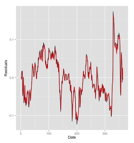
Note that to construct the red line I'm just multiplying the previous day's actual value with the coefficient obtained from the AR1 regression, 0.945.
After getting this, we now obtain the filtered residuals:

And this process turns out to be stationary at the 1% level:

Conclusion
Although AAPL and GOOG are not cointegral in the traditional sense, we can still obtain stationarity in the residuals after filtering for a AR1 process (which we assume to be deterministic). It's interesting to consider if this implies that we can still implement a profitable pairs trade on these two stocks.
Avellaneda and Lee (2008) suggest a trading strategy where we go long on $\text{\$1}$ of AAPL and short on $\beta$ dollars of GOOGL when our stationary residual is low, and vice versa when our residual is high. This means if we are able to predict the cointegration residual, we can make a profitable portfolio.
In the next post I will turn my attention now to modeling and forecasting the cointegration residuals, and backtesting some strategies for AAPL and GOOG.
Aside: Vasicek Model
A popular way to model mean-reverting processes is the Vasicek Model:\begin{align}
dx_t = k(m - x_t)dt + \sigma dW_t
\end{align}
Where $k$ signifies the speed of mean reversion. $m$ signifies the long-run mean, $\sigma$ signifies the instantaneous volatility, and $dW$ is a Brownian motion process. The Vasicek Model belongs to a class of stochastic processes called Ornstein-Uhlenbeck Processes, meaning that they revert to some long-run mean after a while.
We calibrate our above time series to the Vasicek Model. Calibration can be done via Least-Squares. Let's discretize our stochastic differential equation first:
\begin{align}
dx_t &= k(m - x_t)dt + \sigma dW_t \\
x_{t+1} - x_t &= k(m - x_t)dt + \sigma \sqrt{dt} \epsilon_t \\
\epsilon_t &\sim N(0,1)
\end{align}
Now rearrange algebraically,
\begin{align}
\underbrace{x_{t+1}}_{y} &= \underbrace{k*m*dt}_{\alpha} + \underbrace{x_t(1 - k*dt)}_{\beta x} + \underbrace{\sigma \sqrt{dt} z_t}_{\epsilon}
\end{align}
With the last equation we see the linear regression equation. Thus we regress $y_{t+1}$ on $y_{t}$ and retrieve our parameters through the following transformation on our coefficient estimates:
\begin{align}
\alpha &= k*m*dt \\
\beta &= 1 - k * dt \\
\sigma & = \frac{S.D. \epsilon}{\sqrt{dt}}
\end{align}
Vasicek Model Monte-Carlo Simulation
After calibrating the spread to the Vasicek Model with the above procedures, we obtain the following parameters: $k = 9.56$, $m = -0.0037$, $\sigma = 0.206$. We can simulate some realizations of this Vasicek Process to make sure these parameters sound reasonable. The red line is the Monte-Carlo simulation, and the black line is the actual cointegration residual:
The model appears to capture properties of the cointegration residuals fairly well.
References
Avellaneda & Lee. (2008). Statistical Arbitrage in the U.S. Equities Market.
No comments:
Post a Comment